Dynamical Systems, Neural Networks, and TensorFlow

Photo Credit: Mehdi Sepehri
Animal populations can often be described by equations, but not easily predicted by any single formula
See GitHub repo for source code of the signal modeling process and neural network training.
Introduction
Systems in nature, finance, engineering, or anything really, tend to evolve over time. The big question is: can they be reasonably described by a rules-based system?
Such systems are called dynamical systems. They can also be quite complex and unpredictable, though in some cases they can be approximated to some sum of predictable patterns.
Neural networks are able to pick up both simple and complex phenomena while using reasonably generalized training methods, provided they are tuned with some level of expertise.
I decided to build a simulation library for generating signals from dynamical systems, and then predict them using LSTM (long short-term memory) neural networks in TensorFlow.
Dynamical Systems: How do things change?
I’m going to go into a bit more detail on systems changing over time, using some math. If this is confusing, feel free to skip to the section on my applications of neural networks.
Let’s say a system has \(M\) variables \(x_1, x_2, ...x_M\). (I avoid using the letter \(N\) as it denotes the number of time steps in my module.)
We can consider this a dynamical system if the variables’ time derivatives depend on the variables in question:
\[\dot{x}_1 = f(x_1,x_2, ... x_M)\\ \dot{x}_2 = f(x_1,x_2, ... x_M)\\ ...\dot{x}_M = f(x_1,x_2, ... x_M)\\\]My simulation engine can generate signals for any system that can be rewritten in the above form.
Let’s look at an example
Behold, the damped driven oscillator:
Consider an object with mass m attached to a spring with “spring constant” k. There is also a friction constant b which damps the oscillation of the spring. Finally, there is also a driving force \(F(t)\) pushing and pulling on the spring.
Let’s say someone pulls on the mass away from the spring’s equilibrium and lets go, this would lead to a harmonic oscillation, in addition to the driving force.
You will find this situation often written in the following standard form:
\[m\ddot{x} + b\dot{x} + kx = F(t)\]However, we need time derivatives as explicit functions. So we rewrite the above as:
\[\ddot{x} = \dfrac{1}{m}(F(t) - b\dot{x} - kx)\]If we define the mass’s position \(x_1 \coloneqq x\) and the mass’s velocity \(x_2 \coloneqq \dot{x}\), then we essentially have the variables’ time derivatives expressed as functions in the previously mentioned general form:
\[\dot{x}_1 = x_2\\ \dot{x}_2 = \dfrac{1}{m}(F(t) - bx_2 - kx_1)\]How does my simulation engine put these equations into practice?
We first inform the engine initial conditions at time \(t=0\). This includes the mass’s initial velocity \(\dot{x}_{t=0}\) and initial position \(x_{t=0}\). In addition to knowing the driving force at all times, this allows us to calculate the initial acceleration:
\[\ddot{x}_{t=0} = \dfrac{1}{m}(F(t=0) - b\dot{x}_{t=0} - kx_{t=0})\]Then, given a discrete time step size $dt$, use \(\ddot{x}_0\) to calculate the velocity at the next time step:
\[\dot{x}_{t=dt} = \ddot{x}_{t=0}dt\]Repeat this over and over to generate a signal, iterating through values of $t=m\mathrm{d}t$:
\[\dot{x}_{t=(m+1)dt} = \ddot{x}_{t=mdt}\]What does the simulation end up looking like?
Let’s say I’ve got a driving force defined as a sine wave. Perhaps it’s an elf meticulously pushing and pulling on the spring:
\[F(t) = \sin(2\pi t)\]Furthermore I set the initial conditions and constant values as follows:
- mass \(m = 1\)
- friction constant \(b = 0.1\)
- spring constant \(k = 0.1\)
- initial position \(x_{t=0} = 0\)
- initial velocity \(\dot{x}_{t=dt} = 0.5\)
Plugging this into my engine we get the following signal:
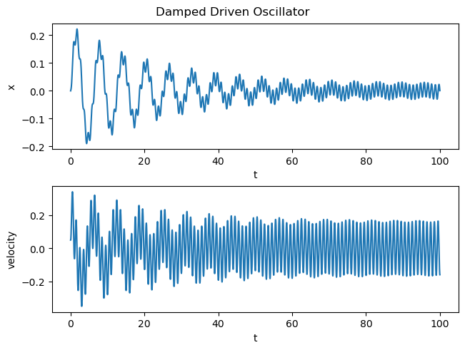
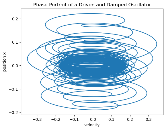
If we plot velocity against position, we can get a more geometric representaion in “phase space”:
How to Use the Engine
Now that we’ve looked at an example, you may be wondering, how do I use the engine to simulate my own nonlinear equation?
The engine revolves around one Python function that I call “x_iterate”. All you need to do is pass the following items (i.e. arguments):
- The initial state vector (1 dimension), which contains the variables’ values at initial time \(t_0\). In the case of the damped oscillator, it would contain initial position \(x_{t=0}\) and initial velocity \(\dot{x}_{t=dt}\).
- The value of the discrete time step \(dt\), i.e. the time of each frame.
- Number of time steps or frames \(N\) for which the simulation takes place
- A list of functions that take calculate the state vector \(x\)’s time derivatives for each variable. For the damped oscillator this would be calculating \(\dot{x}\) and \(\ddot{x}\).
- A dictionary of custom arguments used (if needed) for the functions
How did I use this for my damped oscillator?
I define a function that takes intiial values and constants specific to a damped oscillator and feeds it into the simulation engine.
You will see that functions similar to the above form are created for velocity and acceleration and fed into the the x_iterate function.
def x_driven(x_t0, dt, N, m, b, k, u1, args):
    """
    Description:
        Simulate damped driven oscillator, with driving force u_1(t)
    x_t0: 1 dimensional array (torch tensor), shape n
            contains n values at time t = 0
    dt: scalar value
            timestep quantity
    N: scalar value
        number of time steps to be iterated through
    m: scalar value
        mass constant
    b: scalar value
        friction constant
    k: scalar value
        spring constant
    u: 1 dimensional list, shape n
        contains n functions to be used on x; input functions in a system
    args: dictionary
        arguments for function u
    """
    #Prepare system functions
    #Velocity
    def xdot(x, t, args):
        return x[1]
    #Acceleration
    def xdotdot(x, t, args):
        return (u1(t, args) - b*x[1] - k*x[0])/m

    #Iterate through the time steps to calculate the variables using the system functions
    x_full = x_iterate(x_t0=x_t0, dt=dt, N=N, f=[xdot, xdotdot], args=args)
After importing the library, it’s as simple as using the damped oscillator function. In this case I use a custom function called harmonics which essentially spits out a sum of sine waves (or in this case 1). You can try putting in multiple sine waves of multiple amplitudes and frequencies for fun:
#Import source code
from src import dynamicmodel as dm

#Numeric/Computational libraries
import numpy as np

#Initialize parameters
dt =.02
N = 5000

#Initialize u at t=0
x_t0 = np.array([0,0.05])

x_array_dampeddriven = dm.x_driven(x_t0=x_t0, dt=dt, N=N, m=1, b=0.1, k=1, u1=dm.harmonics, args={'n_list':[1], 'a_list':[1]})
I also used my engine to simulate an RLC circuit, check out the repo to see more!
In this RLC circuit simulation we have:
- The capacitor voltage \(V_C\) with initial value at \(t=0\)
- The inductor current \(I_L\) with initial value at \(t=0\)
- The capacitor’s capacitance \(C\) (defined to be 1 in this simulation)
- The resistor’s resistance \(R\) (defined to be 1 in this simulation)
- The voltage \(V(t)\) from the battery in the circuit, (\(\sin(2\pi t)\) in this simulation)
The system equations are as follows:
\[\dot{V}_C = \dfrac{I_L}{C}\] \[\dot{I}_L = \dfrac{1}{L}(-V_C - RI_L + V(t))\]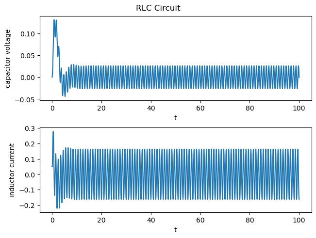
Neural Networks
Do the above examples have clearly discernable patterns? Yes!
Do linear systems in general have clearly discenrable patterns? I think so.
Do complex nonlinear systems have clearly discernable patterns? Sometimes. But that’s another problem for another day.
In any case, a Long Short-Term Memory (LSTM) Neural Network is often used to predict time series. I train an LSTM Neural Network off the dynamical simulation signals and test it’s ability to predict the rest of the signal.
Neural Networks: Training Data
A neural network can’t just be fed some raw signal. It must get proper inputs and outputs.
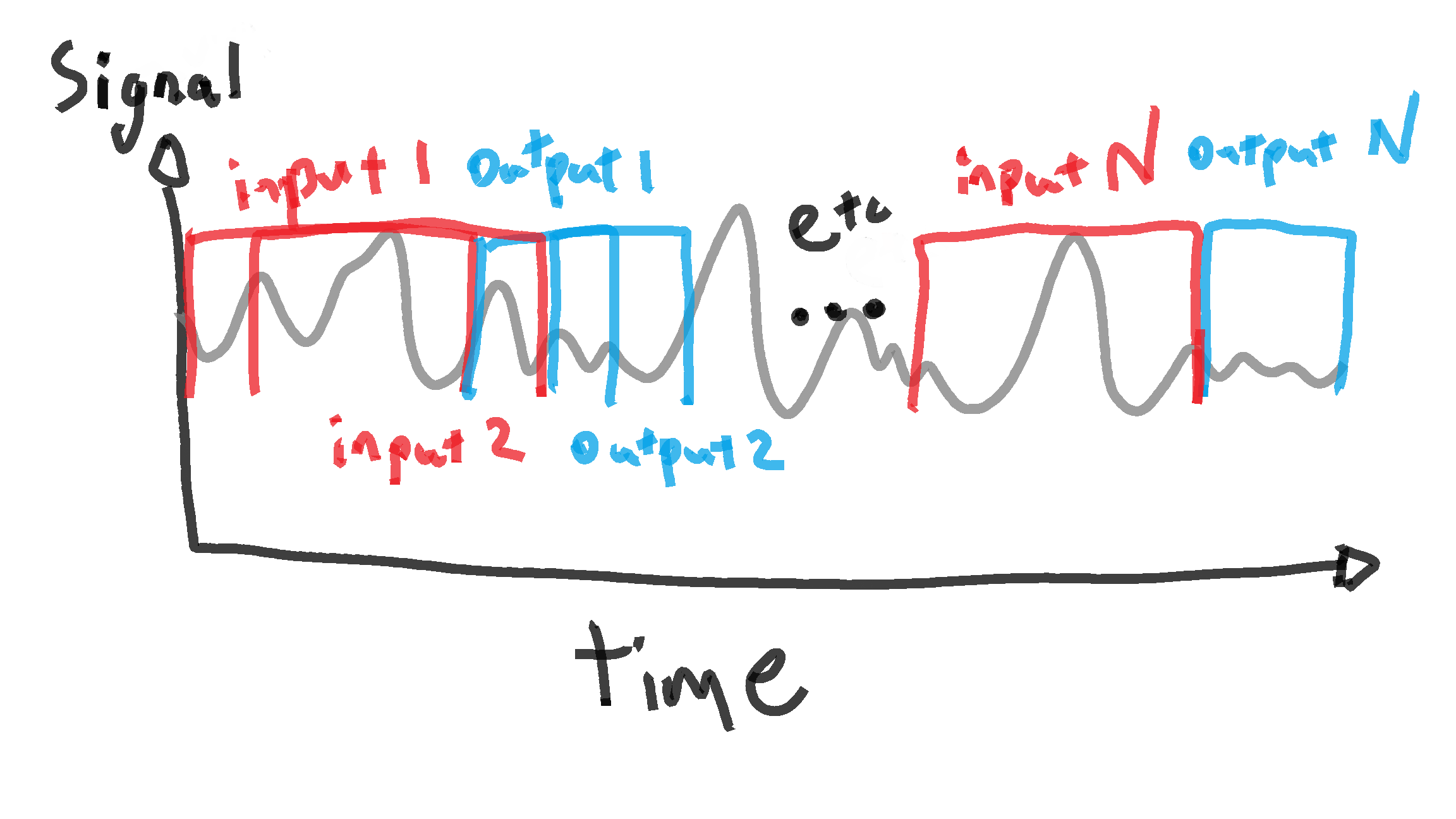
Like my wave simulation prediction project, I use a sort of windowing method to separate the data into neural network inputs and outputs (i.e. labels).
Each “input” window from “n” to “n + n_window” gets a subsequent “output” label from “n + n_window” to “n + n_window + n_predict”.
Code
Here I define a function to format signals into training data:
#Split data into multiple signals (inputs and labels) using a rolling window
def create_dataset(data, n_window, n_predict):
    #initialize data lists
    data_x = []
    data_y = []
    #initialize data
    for n in range(0, len(data)-n_window-n_predict):

        #Get training data
        #Training Inputs
        x = data[n:n+n_window]
        #Training Labels
        y = data[n+n_window:n+n_window+n_predict]

        #append training data and label to final format
        data_x += [x]
        data_y += [y]
    #convert lists to array
    data_x = np.array(data_x)
    data_y = np.array(data_y)
    return data_x, data_y
Neural Networks: Training and Tensorflow
First I split the signals into training and test data. The test data comes after the training part of the signal, and is a hold out to compare to the neural network’s predictions.
After I format the “training” part of the signals, all that’s left to do is to create neural networks that learn off the training data.
This is relatively simple in Keras (in the TensorFlow platform). I create a neural network with one LSTM layer and optimize it using mean squared error. Each model is trained through the entire training section of the signal once, using the overlapping window method.
Code: Note that these are just illustrative snippets of code. For entire context see repo.
Here the create_dataset function is deployed to prepare training data off of the Pandas DataFrames df1 and df2, which contain the previously generated signals:
#Determine length of training data
len_train = 4000

#Apply window function to prepare training data
n_window=200
n_predict=1
#damped oscillator data
x_train1, y_train1 = create_dataset(data=df1['x'].to_numpy()[0:len_train], n_window=n_window, n_predict=n_predict)
#rlc circuit data
x_train2, y_train2 = create_dataset(data=df2['capacitor voltage'].to_numpy()[0:len_train], n_window=n_window, n_predict=n_predict)

#Reshape input to be [samples, time steps, features]
x_train1 = np.expand_dims(x_train1, axis=1)
x_train2 = np.expand_dims(x_train2, axis=1)
Here I define a simple function to create a neural network with one LSTM layer so that I don’t have to repeatedly write the same 4 lines of code.
That being said, TensorFlow’s Keras interface is very simple.
I only need to specify the input size and output size and call some functions to add layers.
def create_model(x_length, y_length):
    """
    Description:
        Create an LSTM model with specific parameters

    Args:
        x_length: int, length of training inputs
        y_lenght: int, length of training outputs
    """
    model=tf.keras.models.Sequential()
    model.add(tf.keras.layers.LSTM(units=n_predict, input_shape=(x_length, y_length)))
    model.add(tf.keras.layers.Dense(1))
    model.compile(loss='mean_squared_error', optimizer='adam')
    return model
Here I just create the neural networks and then train them off the training data.
#Determine model parameters
x_length = 1
epochs = 15
batch_size = 1

#Create neural networks as Tensorflow model objects
model1 = create_model(x_length=x_length, y_length=n_window)
model2 = create_model(x_length=x_length, y_length=n_window)
#Train Model
model1.fit(x_train1, y_train1, epochs=epochs, batch_size=batch_size, verbose=2)
model2.fit(x_train2, y_train2, epochs=epochs, batch_size=batch_size, verbose=2)
Neural Networks: Predictions
You may have noticed that I set the prediction size to 1. How do we have the neural networks predict a reasonably long signal with just size 1?
Let’s say we take the last “n_window” samples from the signal and make a prediction of size 1 after that. Then we can simply add that prediction to the input and move the window forward one sample in time. Do this repeatedly until you’re happy with the length of the predicted signal.
This is how I make predictions with the LSTM neural network off the signal.
To see how the prediction process is specifically deployed please see the repo.
Let’s see how the predictions look!
Below we have plots of the generated signals (training data), the neural networks predictions on how the signal will evolve, and how the signal actually evolves.
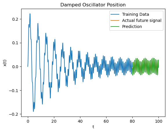
Above we have the damped oscillator. The prediction seems to be capturing the damping phenomena, driving frequency, and spring force frequency well.
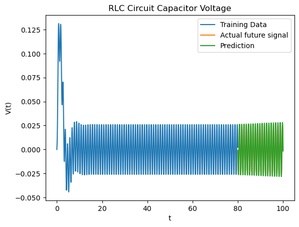
Above we have an RLC circuit. Actually, once the signal stabilizes there’s really not much nuance: just one single oscillation. As expected, the neural network predicts the voltage perfectly.
What Next?
Nonlinear Dynamics
So far we’ve simulated and predicted some reasonably simple linear phenomena. Everything that occured in the signals was easily explanable, and was more or less picked up by the neural network, albeit not perfectly.
But the dynamic modeler engine can simulate much more complex nonlinear phenomena provided they fit into the same dynamical format. Perhaps this may include coupled oscillators or nonlinear circuit voltages.
Signal Processing
It’s often the case that a bit of preprocessing buys machine learning a lot of accuracy.
Given that there is often phenomena happening at different frequencies, I may try band-pass filtering the signal into multiple signals, feed the signals into multiple neural networks, and add the predictions back together.